Extending the Latent Uniformly

To explain the “Extending the Latent Uniformly” trick I used to boost visual consistency in FIFO-Diffusion, we need to dive into the mechanism behind long video generation.

• FIFO-Diffusion: Generating Infinite Videos from Text without Training

Background

FIFO-Diffusion is a train-free method built on fixed-length, pre-trained video diffusion models.

1. Base model generates a video \(\mathbf{v}\in \mathbb{R}^{f\times H \times W \times 3}\).
   • \(f\) is the number of frames
   • \(H\) and \(W\) are the height and width of a frame, the pixel resolution
   • \(3\) is the number of color channels (RGB)
   • Example: VideoCrafter’s 320x512 model \(\mathbf{v}\in\mathbb{R}^{16\times 320 \times 512 \times 3}\)

   

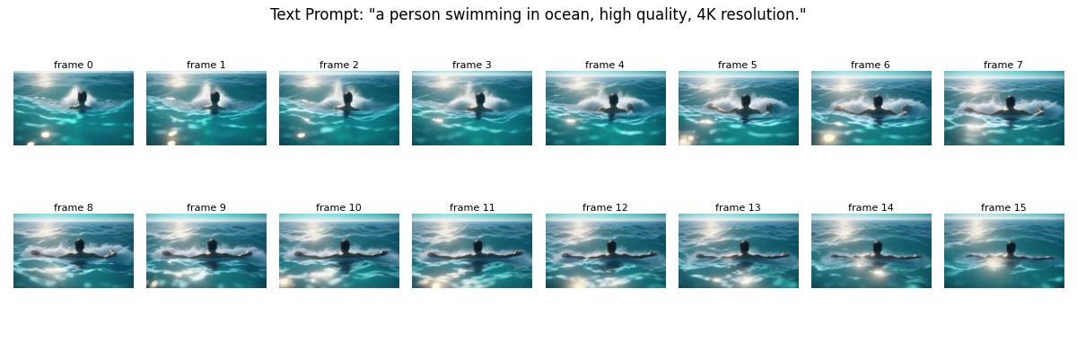
2. An autoencoder encode a video \(\mathbf{v}\) into a video latent \(\mathbf{z_0}=\text{AutoEnc}(\mathbf{v})\).

   • A (clean) video latent \(\mathbf{z_0} = [z^1_0;...;...z^f_0]\in \mathbb{R^{f\times h \times w \times c}}\)
   • \(h\) and \(w\) are the height and width of the feature map
   • \(c\) is the number of channels
   • Dimensionality reduction by \(\text{AutoEnc}: \mathbb{R}^{16\times 320 \times 512 \times 3} \rightarrow \mathbb{R}^{16\times 40 \times 64 \times 4}\)

3. The forward process transitions a clean latent \(\mathbf{z_0}\) to a noisy latent \(\mathbf{z_t}\) by progressively adding Gaussian noise at each timestep.

   \[\mathbf{z_t}=\sqrt{\alpha_t}\mathbf{z_0}+\sqrt{1-\alpha_t} \epsilon, \text{ where } \epsilon \sim \mathcal{N}(0, \mathbf{I})\]

   where \(\alpha_t \in (0, 1)\) is a linearly decreased coefficient. If expressed in frame vector, for a timestep \(t\):

   \[\begin{bmatrix}z^1_t\\z^2_t\\ \vdots\\ z^f_t\end{bmatrix} = \sqrt{\alpha_t} \begin{bmatrix}z^1_0\\ z^2_0\\ \vdots\\ z^f_0 \end{bmatrix} + \sqrt{1-\alpha_t} \epsilon\]

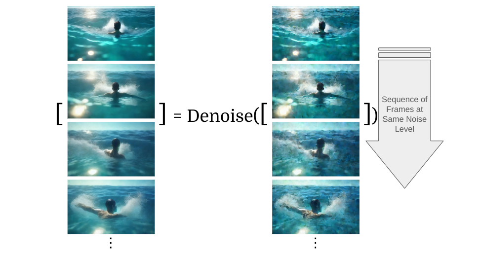
4. The denoising process transitions a noisy latent \(\mathbf{z_t}\) to a cleaner version \(\mathbf{z}_{t-1}\).

   \[\begin{bmatrix}z^1_{t-1}\\ z^2_{t-1}\\ \vdots\\ z^f_{t-1} \end{bmatrix} = \text{Denoise}\Bigl(\begin{bmatrix}z^1_t\\z^2_t\\ \vdots\\ z^f_t\end{bmatrix}\Bigr)\]

   Visually speaking, it’s like this image — though I’ve exaggerated the noise difference here to make it easier to see:

---

Key to infinite video generation: Diagonal denoising & Queue

In diagonal denoising, the input noisy latent \(\mathbf{z}^{\text{diag}}_t\) no longer has all its elements at the same noise level. Instead, each component is perturbed to varying degrees.

\[\begin{bmatrix}z^1_{t-1}\\ z^2_{t}\\ \vdots\\ z^f_{t+f-1} \end{bmatrix} = \text{Denoise}\Bigl(\begin{bmatrix}z^1_{t}\\z^2_{t+1}\\ \vdots\\ z^f_{t+f}\end{bmatrix}\Bigr)\]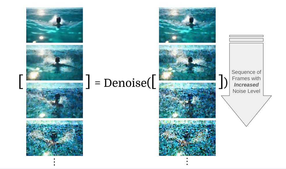

FIFO-Diffusion uses a queue to keep track of the latent frames. After each denoising round, the first latent frame in the queue becomes the cleanest. This cleanest frame is then dequeued, making space for a new one, which we enqueue a standard Gaussian noise \(z \sim \mathcal{N}(0, 1)\). The whole process works like this figure:

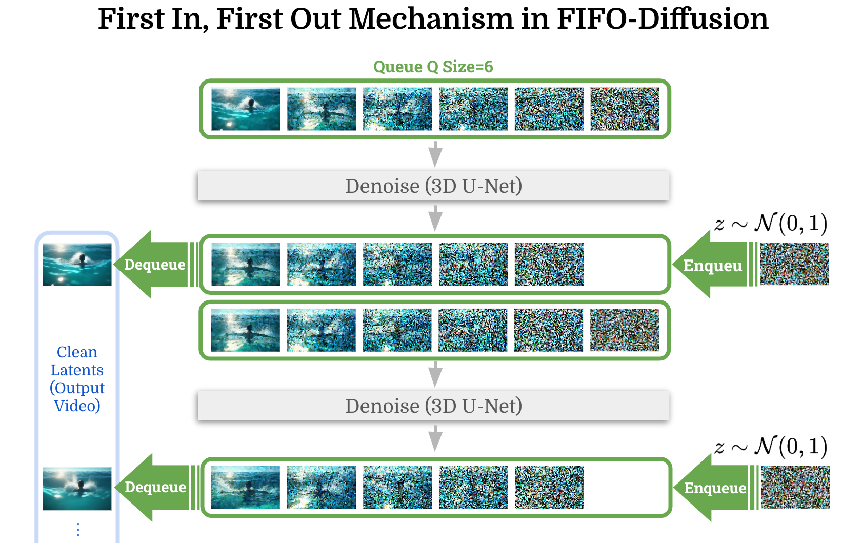
By combining a first-in, first-out queue with diagonal denoising, they achieved infinite video generation!

But here’s the twist: the denoising network is actually trained to remove noise at a specific level. So, in a way, this approach is kind of a “misuse” of the network’s original purpose. The author does back it up with theoretical proof, which states that:

the gap incurred by diagonal denoising is linearly bounded by the maximum noise level difference, implying we can reduce the error by narrowing the noise level differences of model inputs.

Reducing the Noise Differences

FIFO-Diffusion uses two strategies to reduce noise discrepancies: Latent Expending and Latent Partitioning. And there are a couple of requirements to keep in mind:

• We need enough inference steps to balance image quality and computational efficiency.
• Matching the base model’s input temporal length.

The base model, VideoCrafter, uses a DDPM scheduler with 64 inference steps. Think of it like a 64-step guide to gradually removing noise from a video. And a denoising U-Net with the temporal length 16.

Latent Expending

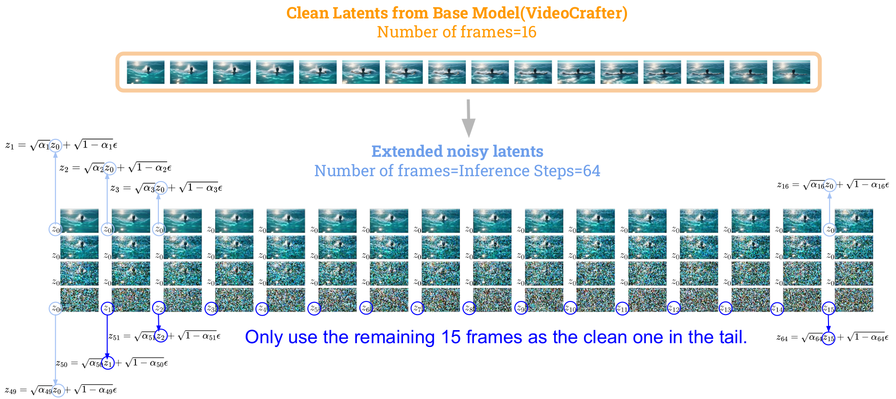
Inference steps means that there is a sequence of \(\alpha_t\), where \(t \in {1,...,64}\). These values determine how much noise is added at each step given a clean \(z_0\):

\[\mathbf{z_t}=\sqrt{\alpha_t}\mathbf{z_0}+\sqrt{1-\alpha_t} \epsilon, \text{ where } \epsilon \sim \mathcal{N}(0, \mathbf{I})\]

When we talk about the 64 levels of noise perturbation, it means that for each noise level, there’s a corresponding clean latent \(z_0\) as well, but the base model only gives us 16. The authors don’t explicitly mention how they did it, but they included the details in their code.

def prepare_latents(args, latents_dir, sampler):
...
for i in range(args.num_inference_steps):
    alpha = sampler.ddim_alphas[i] # image -> noise
    beta = 1 - alpha
    frame_idx = max(0, i-(args.num_inference_steps - args.video_length))
    latents = (alpha)**(0.5) * video[:,:,[frame_idx]] + (1-alpha)**(0.5) * torch.randn_like(video[:,:,[frame_idx]])
    latents_list.append(latents)
...

The default latent expansion behavior fills most of the space with the first latent (frame 0 \(z_0\)) as its clean latent and only uses the remaining frames (frame 2-16, \(z_{2-16}\)) towards the end. As you can see in the figure below, the left bottom \(z_i\) is its corresponding clean latent.

Latent Partitioning

In fit U-Net’s temporal length f=16(VideoCrafter). They partition the extended latent (length=64) into segments with length 16, then each partition can be denoised independently. The whole procedure, along with the enqueue/dequeue mechanism, works like this:

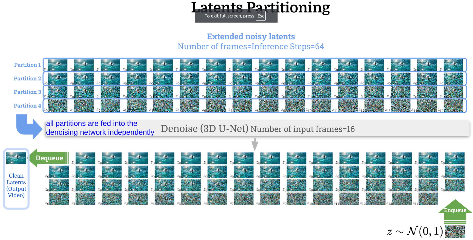
Another great benefit of partitioning is that it significantly cuts down the noise difference. Instead of having a huge noise gap between the 1st and 64th latent, it’s now just between the 1st and 16th!

My Observation and Improvements

After watching a bunch of videos generated by FIFO-Diffusion, I noticed that the longer the video, the more unstable it got. I suspect this is because the default latent expansion makes the last partition (partition 4) quite different from the earlier ones (partitions 1-3), as shown in this figure:

So, I gave it a try by extending the latent uniformly.

I’m impressed with how well this experiment turned out!

Results

FIFO-Diffusion	+ Q-Caches	+ Q-Caches + Uniform Latent
"a person swimming in ocean, high quality, 4K resolution."

Erroneous segment: The body morphs from the back to the front.

Improved Segment (Frame 119-136)

---

FIFO-Diffusion	+ Q-Caches	+ Q-Caches + Uniform Latent
"an airplane accelerating to gain speed, high quality, 4K resolution."

Erroneous segment: Airplane morphs toward different direction.

Improved Segment (Frame 73-82)

---

FIFO-Diffusion	+ Q-Caches	+ Q-Caches + Uniform Latent
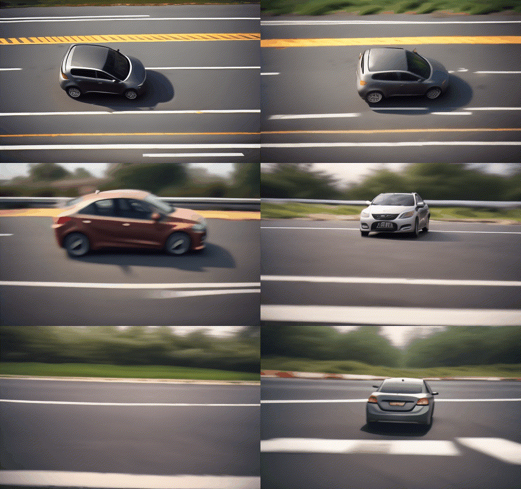
"a car slowing down to stop, high quality, 4K resolution."

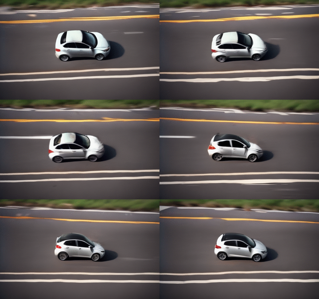
Erroneous segment: Car roof swaps to black.

Improved Segment (Frame 106-114)

More camera movements.

FIFO-Diffusion	+ Q-Caches	+ Q-Caches + Uniform Latent
"a person giving a presentation to a room full of colleagues, high quality, 4K resolution."

---

Quick note:

• When I mention the “Denoising Process” here, I’m using it as an umbrella term. Technically, calling it a noise prediction process is more accurate, as it predicts the noise level in a perturbed latent.

• I’m skipping over Lookahead Denoising mechanism in this series since I want to keep things simple for now. If you’re curious, check out the original paper for the details.